Recent trends in cabinet size
The average number of parties in government peaked in the last decade
Many countries are governed by one multiple political parties at the same time. Indeed, the number of parties in government — the cabinet size — is rarely one.
In this blogpost, I explore the average cabinet size, and how this average has been trending in the recent history.
To do so, I turn to the Parliaments and Governments Database (ParlGov), which brings together three inter-related datasets, as presented in Table 1. Here I work with only one of them: Cabinet.
| Dataset | Filename | Observations |
|---|---|---|
| Parties | view_party | 1700 |
| Elections | view_election | 1000 |
| Cabinets | view_cabinet | 1600 |
To start with, let’s load three packages that I need for this task, dataverse (to download the dataset from Harvard Dataverse), tidyverse (to clean, tidy, and plot the data), and knitr (to table the data).
I will leave the underlying R code visible, in case you are interested in this sort of thing.
# load the packages needed

library(dataverse)
library(tidyverse)
library(knitr)
We can now download the dataset with the get_dataframe_by_name function.
# download the data from harvard dataverse

df_cabs <- get_dataframe_by_name(
  filename  = "view_cabinet.tab",
  dataset   = "10.7910/DVN/Q6CVHX",
  server    = "dataverse.harvard.edu"
  )
How does the dataset look? We can use the kable function function to see. However, this is a large dataset. As of 25 April 2021, it has 12070 observations and 19 variables. Therefore, Table 2 displays only a random selection of these observations.
# table a random selection of observations

kable(sample_n(df_cabs, 10),
caption = "Randomly selected 10 observations in the Cabinet dataset")| country_name_short | country_name | election_date | start_date | cabinet_name | caretaker | cabinet_party | prime_minister | seats | election_seats_total | party_name_short | party_name | party_name_english | left_right | country_id | election_id | cabinet_id | previous_cabinet_id | party_id |
|---|---|---|---|---|---|---|---|---|---|---|---|---|---|---|---|---|---|---|
| HUN | Hungary | 1998-05-24 | 1998-07-06 | Orban I | 0 | 1 | 1 | 148 | 386 | Fi-MPSz | Fidesz – Magyar Polgári Szövetség | Fidesz – Hungarian Civic Union | 6.5432 | 39 | 671 | 827 | 488 | 921 |
| AUS | Australia | 2016-07-02 | 2016-07-19 | Turnbull II | 0 | 1 | 1 | 45 | 150 | LPA | Liberal Party of Australia | Liberal Party of Australia | 7.3903 | 33 | 1006 | 1490 | 1174 | 1411 |
| TUR | Turkey | 1995-12-24 | 1997-06-30 | Yilmaz III | 0 | 0 | 0 | 158 | 550 | RP | Refah (Fazilet) Partisi | Welfare (Virtue) Party | 8.3333 | 20 | 810 | 1099 | 1098 | 1122 |
| DEU | Germany | 1930-09-14 | 1930-12-05 | Brüning III | 0 | 0 | 0 | 4 | 577 | KVP | Konservative Volkspartei | Conservative Peoples’ Party | 7.4000 | 54 | 1037 | 1583 | 1582 | 2711 |
| ISR | Israel | 1996-05-29 | 1996-06-18 | Netanyahu I | 0 | 1 | 0 | 5 | 120 | Gesher | Gesher | Bridge | 7.4000 | 34 | 717 | 961 | 960 | 1862 |
| ISR | Israel | 1949-01-25 | 1950-11-01 | Ben-Gurion III | 0 | 0 | 0 | 7 | 120 | ZK | Zionim Klalim | General Zionists | 6.0000 | 34 | 704 | 923 | 922 | 1472 |
| CZE | Czech Republic | 1996-06-01 | 1998-01-02 | Tosovsky | 1 | 0 | 0 | 61 | 200 | CSSD | Ceská strana sociálne demokratická | Czech Social Democratic Party | 3.0463 | 68 | 301 | 76 | 136 | 789 |
| DNK | Denmark | 1947-10-28 | 1947-11-13 | Hedtoft I | 0 | 0 | 0 | 6 | 150 | RF | Retsforbund | Justice Party | 6.0000 | 21 | 541 | 408 | 387 | 1606 |
| DEU | Germany | 1930-09-14 | 1930-12-05 | Brüning III | 0 | 0 | 0 | 107 | 577 | NSDAP | Nationalsozialistische Deutsche Arbeiterpartei | National Socialist German Workers’ Party | 8.8000 | 54 | 1037 | 1583 | 1582 | 2695 |
| ISR | Israel | 1992-06-23 | 1995-11-22 | Peres II | 0 | 0 | 0 | 1 | 120 | none | no party affiliation | no party affiliation | NA | 34 | 716 | 960 | 1120 | 123 |
Before visualising the trend over the years, we need to get the data into the right shape. There are many helpful functions in the tidyverse family for this purpose.
# tidy the data

df_ends <- df_cabs %>%
        filter(start_date > as.Date("1948-12-31") & start_date < as.Date("2020-01-01")) %>%
        mutate(end_year = as.numeric(format(start_date,'%Y'))) %>%
        select(previous_cabinet_id, end_year) %>%
        distinct()

df <- df_cabs %>%
      filter(start_date > as.Date("1948-12-31") & start_date < as.Date("2020-01-01"))  %>%
      mutate(start_year = as.numeric(format(start_date,'%Y'))) %>%
      group_by(cabinet_id, start_year) %>%
      summarise(parties = sum(cabinet_party)) %>%
      ungroup() %>%
      left_join(., df_ends, by = c("cabinet_id" = "previous_cabinet_id")) %>%
      mutate(end_year = replace_na(end_year, 2019)) %>%
      pivot_longer(cols = c("start_year", "end_year"), values_to = "year") %>%
      select(-name) %>%
      group_by(cabinet_id) %>%
      complete(cabinet_id, year = full_seq(year, 1)) %>%
      fill(parties) %>%
      group_by(year) %>%
      summarise(cabinet_size = mean(parties))
Now that the data is in the right shape, Figure 1 plots it.
# plot the data

ggplot(df, aes(x = year, y = cabinet_size)) +
        geom_line(size = 1.5) +
        theme_minimal() +
        theme(axis.title = element_text(size = 14),
              axis.text = element_text(size = 14)) +
        labs(y = "Average cabinet size\n", x = "")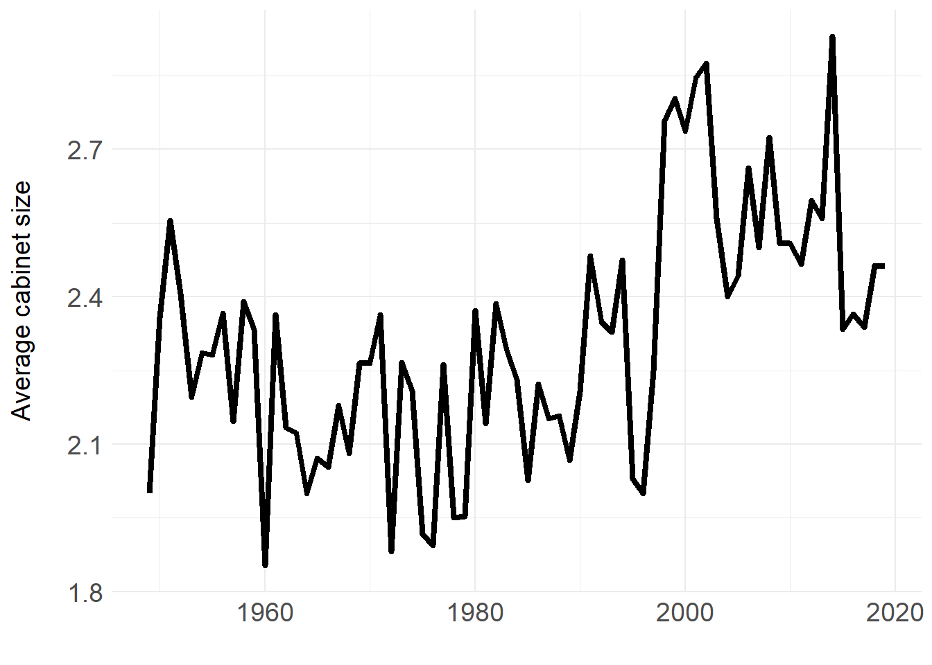
Figure 1: Average cabinet size, 1949–2019.
The figure shows that the average number of parties in government peaked in the last decade.
Jane J. Doe
Associate Professor of Politics
My academic interests include party politics, public policy, and international polities.